9.1: Memory management
In the previous chapters we have many times talked about (RAM) memory and (RAM) memory addresses, as well as specialized memory regions such as the stack and the heap. Up until now, we have pretended as if these concepts mapped directly onto the underlying hardware, but reality is of course a bit more complex. In this chapter, we will consider how physical memory is actually managed by the OS and the CPU.
Memory addresses and address lengths
In modern computers and embedded systems there is typically a large amount of memory available. To be able to read and write to this memory, we need a way to access individual units of storage. This is done using memory addresses, numbers that uniquely identify memory locations. In theory, we could assign an address to each individual bit of physical memory, but in practice we address groups of 8 bits (or 1 byte). This means we always read/write 8 bits at a time. This is firstly because we don’t often work with individual bits and secondly because more addresses means more overhead, as we will soon see.
How many individual bytes we can support depends on how long our address numbers are. For example, a relatively simple/embedded system like the ATMega 328p on the Arduino Uno, has an address length of 8 bits. Consequently, this chip is said to be an 8-bit processor. 8 bits worth of addresses gives us 28 = 256 individual memory locations of 8 bits each, so a total of 256 bytes (not exactly a lot).
For a long time, more complex chips and general purpose CPU’s were 32-bit. This allows for a maximum of 232 = 4.294.967.296 individual bytes to be addressed. This comes down to about 4 GigaBytes of memory. For a long time, this was sufficient, as (RAM) memory was almost always (much) smaller than 4GB. However, as we know, over time memory was made that could be much larger than that, meaning that 32-bit processors were no longer enough.
This is when the big switch to 64-bit processors happened. This allows for a maximum of 264, which is equivalent to 224+10+10+10+10, which means 224 terabyte or 16 exabyte. The expectation is that that will remain enough for quite a while ;)
You might notice that, especially for 64-bit, there won’t always be enough physical memory to back the entire addressable space. As we will see later, this is where virtual memory addresses come in. To get there however, we need to introduce a few concepts first.
Option 1: Chunking
On small systems-on-chip (SOCs) that do not run an operating system, the world of memory addresses looks flat (starting at 0x00 and ending at 0xFF). Your singular program has full and direct access to the entire memory. However, as we’ve seen many times, one of the key purposes of an OS is to provide the ability to run multiple different tasks on shared hardware. As such we somehow need to subdivide the available memory amongst these tasks.
The OS then mainly has to make sure that process A doesn't try to address memory of process B and vice versa. Often this is referred to as memory protection.
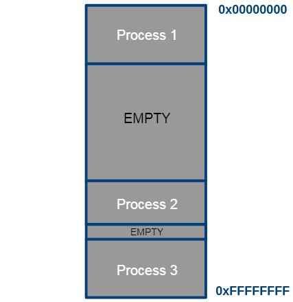
The complete memory space, divided to one chunk per process.
This approach can be easily implemented in hardware with two registers. When a process is scheduled, the OS loads the CPU base register and the limit register with the correct values. The CPU can then check that the addresses of all memory accesses fall within the interval of the base address PLUS the limit. If this condition does not hold, there might be an (un-)intentional error. The CPU propagates this error to the OS for handling.
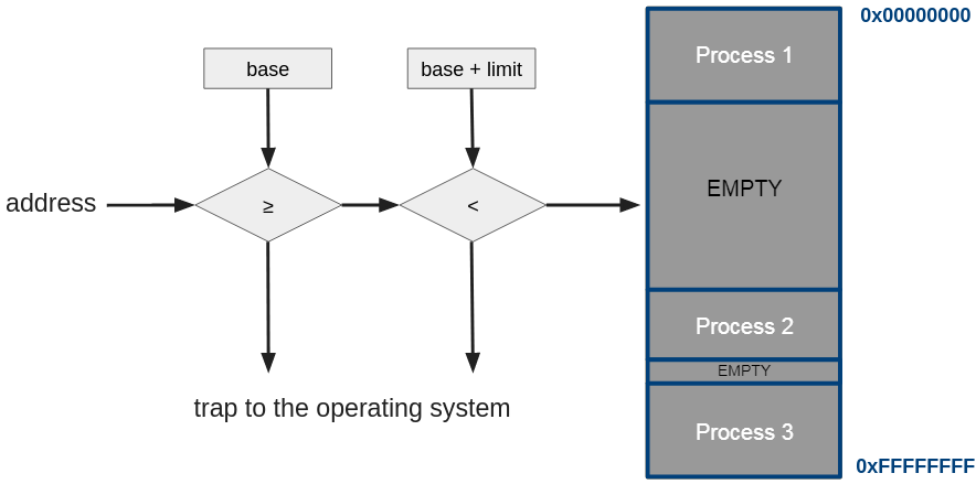
Base address register and limit register in logical addressing.
Importantly in this design, the two CPU registers that store the base and limit values should only be written by processes from the OS’s kernel-space, for example by employing a special privileged instruction.
Address Binding
With this simple approach, let’s consider how memory addresses can be assigned to programs/processes in practice. This is important, as each variable/function in a program needs to reside at a specific address so it can be used/called. For example, assembly doesn’t call functions by their name like C, but by the address at which that function’s instructions start. As we’ve seen earlier, in a modern CPU architecture, code is stored in the same way as data (the text/data/bss segments).
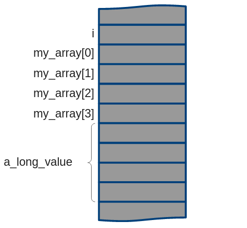
Consider for example the following code, which includes some variables. These variables need to be somehow assigned one or more addresses in the memory for the running process:
      #include <stdio.h>

      int main(void) {
        short i;
        short my_array[4];
        long a_long_value;
        ...
      }
The question is then for example: at which address does the value for `i` begin?
We can see that with chunking, the address space for a certain program can (and will) be different for each run of the program, as the chosen chunk won’t always be at the same place in memory. As such, we cannot assign these addresses at compile time for example, as the compiler won’t know where exactly the program will be loaded (and we cannot expect the OS to load a given program at the same place all the time). Additionally, the compiler also won’t have full information about everything the program needs: for example, a program can load external software libraries, whose details are not yet known at compile time (and are for example resolved (mostly) at link time).
As such, this memory mapping needs to be done at load time, when the OS takes a program and turns it into a process instance. However, for the compiler to generate assembly instructions, it still needs to know the addresses of the variables/functions, as we’ve said above! It seems we have a contradiction here…
The way this is solved, is by having the compiler generate relative/logical/virtual addresses. The compiler for example pretends that the program will always be loaded at address 0x0 and places all variables/functions relative to 0x0. Then, when the program is executed, the addresses can just be incremented with the process chunk’s base address to get the real, physical address in RAM (so physical adress = compiler-generated/logical/virtual address + base address).
As such, we can see that we have two different address spaces: the logical/virtual address space (always starting at 0x0 for each process) and the physical address space (where each process starts at a different offset).
In practice, this can even be done in hardware outside of the CPU, where a separate chip, the so-called “Memory Management Unit” (MMU), takes care of the translation. Using virtual/logical addresses at the CPU then simply requires the use of a relocation register (which can be loaded with the chunk’s base address) to obtain the final physical address:
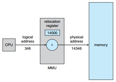
The MMU
source: SILBERSCHATZ, A., GALVIN, P.B., and GAGNE, G. Operating System Concepts. 9th ed. Hoboken: Wiley, 2013.
Problems with Chunking
Chunking and load-time address binding works, but it has some downsides. For example, we would need to know all the variables/functions that will be used at load time. While we know more about them than at compile time (as the link step is done now), we often still don’t know everything yet. This is for example the case when using dynamically loaded external software libraries (so-called “dynamically linked libraries” or DLLs), which is something you typically do want to enable broad code re-use. These DLLs can be loaded during the execution of a process as needed, which is later than the load time we’ve considered.
A more important downside of chunking however is that we would have to assign a fixed-size chunk to each process. This isn’t so much a problem for text/data/bss/stack, but more for the heap. We don’t really know how much heap memory a program will want to use up front, and this often also depends on how the program is used (sometimes you’ll use less memory, sometimes more). You can’t also just give each program a huge amount of memory (say 1GB of heap), as that would severely limit the amount of processes you could run at the same time. As such, you would again have to rely on the programmer to somehow give an indication of program size, or for example learn it from previous executions of the program.
Finally, there is the problem of external fragmentation. As more and more programs are loaded into memory, the available space is reduced. Luckily, as programs are stopped/done, they also release the space they took up. As such, after a while, there will be gaps in the physical memory where older programs were removed. The thing is: those gaps are not always large enough to entirely fit a newly started program! As such, even though conceptually there is enough memory free when we regard the entire memory space, there is not enough -contiguous- memory to fit a new process. This is called “external” fragmentation, as the fragmentation happens outside of the space allocated to processes. We will discuss internal fragmentation later.
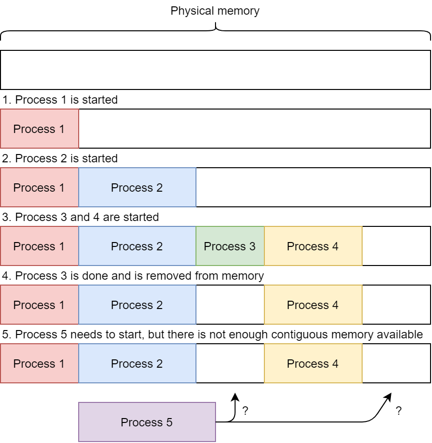
External fragmentation with chunking
It is clear we need a more advanced setup in practice.
Option 2: Segmentation
Segmentation is a more flexible way than chunking of loading processes into memory. The concept of segmentation is pretty simple: instead of reserving a single, large chunk for each process, we will instead reserve several, smaller chunks (called segments). For example, we can have a chunk for the text section, for data, bss, and the stack. And then we can have one (or more!) segments for the heap.
This nicely solves the problems of chunking: we can now appropriately size segments when loading new libraries/DLLs at runtime and we don’t need to reserve huge amounts of memory for each process up-front: we can just add (and remove!) segments as needed!
Additionally, it provides us with extra benefits, such as the fact that the segments for a single process no longer need to be in contiguous memory blocks!. This is illustrated by the images below:

Continuous image: the logical address space of a process. Source: G.I.

Segmented image: the physical address space in which the process' chunks can be located in different areas.
This is a very important characteristic, as it helps deal with the aforementioned external fragmentation (at least up to a certain point). Even though the full process cannot fit in any given gap, its individual segments can be distributed across several gaps as needed.
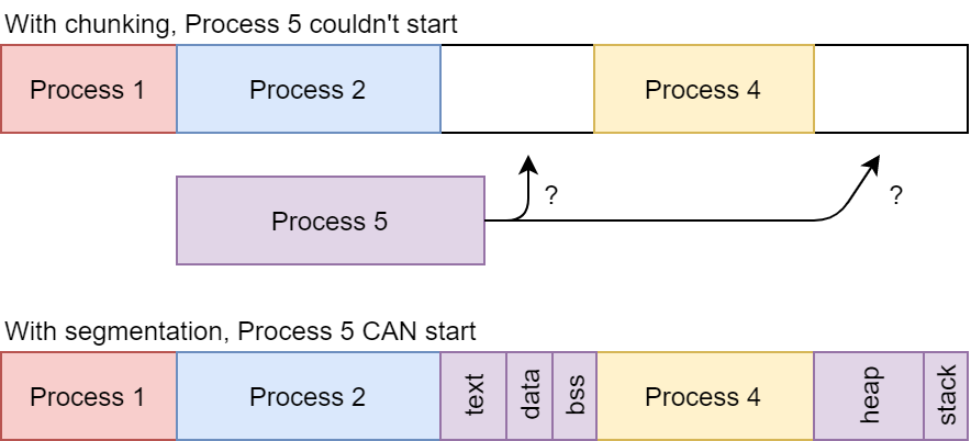
External fragmentation is partially solved with segmentation
Address Binding
Additionally, segmentation allows us to do the memory mapping not at load time (as with chunking), but also much more dynamically at execution time: segments can be created (or removed) and placed as-needed by the OS.
However, placing multiple segments at various locations in the physical memory does mean it now becomes more difficult to find the correct physical address given a logical/virtual address. A single relocation register is no longer enough (as we also no longer have a simple base address). Instead, we need a segment table that tracks the different segments and where exactly they can be found in physical memory. So, instead of having a single base address and a chunk limit, each individual segment has its own base address and limit offset, all of which are stored in the segment table. Again, for performance reasons this is often done in the separate MMU chip, which might look a bit like this:
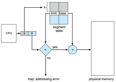
Segmentation hardware
source: SILBERSCHATZ, A., GALVIN, P.B., and GAGNE, G. Operating System Concepts. 9th ed. Hoboken: Wiley, 2013.
This also means that we no longer have a single contiguous logical/virtual address space, but instead multiple smaller ones (one for each segment). In practice, we can still represent addresses with a single number however, which secretly consists of two parts: a segment number (s) and an offset (d). The segment number (s) will be used as an index into the segment table. The value at that index indicates the base address of that segment. The offset number (d) will be used to define an offset within this segment and is simply added to the base address to get the final, physical address.
As with chunking, if the sum of the base address and the offset falls within the segment limit, everything is fine. Otherwise the operating system will catch this error.
What, oh what, could be the name of the error that the OS produces if the sum of the base address and the offset does not fall within the segment limit ?
Problems with Segmentation
While segmentation already improves a lot on chunking, it still suffers from a few problems.
In practice, external fragmentation can still easily occur in modern systems with hundreds of running processes. This is because the individual segments are not equally sized, and gaps (created by removed/stopped segments) can thus easily be smaller than what is needed for a given segment. As such, the OS needs to keep track of a list of open gaps and their size. Every time a process needs memory for a segment, the OS would need to loop over the entire gap list to determine the most appropriate one, a list which can get very long quite quickly. This overhead can get quite substantial in practice. The OS could instead optimize and look for a “good enough” gap, but this in practice only worsens external fragmentation. Other techniques can be considered, such as compaction: this would “shift” segments of running processes together in memory to fill smaller gaps, making larger gaps available. While possible, this can get highly complex, as the logical addresses would also have to be re-generated.
As such, even segmentation isn’t our “final solution” to this problem. But before we discuss the real deal, let’s do some exercises.