7.1: Scheduling algorithms
In the previous chapter on Tasks, we’ve discussed one of the main responsibilities of an operating system: task management. Well to be fair, we have only been creating tasks and stopping or killing tasks. The necessary component that allows tasks to be run on one or multiple processors, the scheduler, is discussed in this chapter. Note that “tasks” or “jobs” can refer to either processes and/or threads.
The scheduler has two main responsibilities:
- Choose the next task that is allowed to run on a given processor
- Dispatching: switching tasks that are running on a given processor
Remember the image below? The first responsibility of the scheduler is the transition between the “ready” and “running” states by interrupting (pausing) and dispatching (starting/resuming) individual tasks:
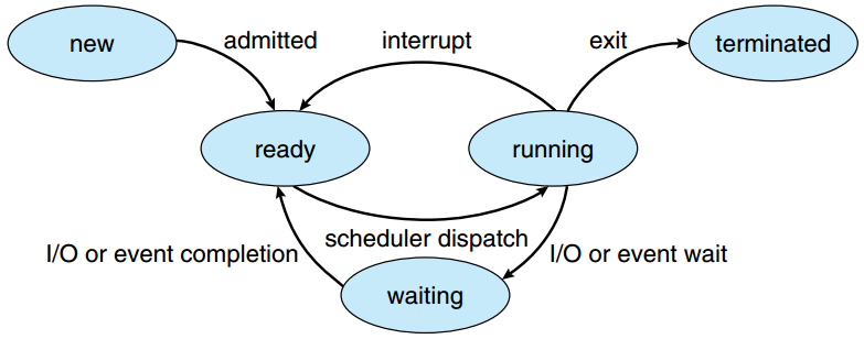
The different process states and their transitions
source: SILBERSCHATZ, A., GALVIN, P.B., and GAGNE, G. Operating System Concepts. 9th ed. Hoboken: Wiley, 2013.
While the image above is mainly for processes, similar logic of course exists for Threads as well, as they go through similar conceptual lifecycle phases as processes.
For the sake of simplicity, in this chapter we assume a system which has only a single processor with a single CPU core. However, the concepts introduced here also (largely) hold for multi-core systems.
(Don’t) Interrupt me !!
When working with a single core, only a single task can be active at the same time. Say that the scheduler starts with the execution of the first task. It then has two options to determine when the next job is dispatched:
- non-preemptive / cooperative scheduling: Let the current task run until it is finished or until it (explicitly) yields (to give up/away, to release) its time on the processor. One way of yielding is for example by using the
sleep(), but alsopthread_join()orsem_wait()can indicate a task can be paused for the time being. - preemptive scheduling: Interrupt the current task at any time. This is possible because the PCB and equivalent TCB’s track fine-grained per-task state.
While the cooperative scheduling approach is the simplest, it also has some severe downsides. If a given task takes a long time to complete or doesn’t properly yield at appropriate intervals, it can end up hogging the CPU for a long time, causing other tasks to stall. As such, most modern OSes will employ a form of preemptive scheduling.
If the scheduler needs to preempt jobs after a certain amount of time (or execution ticks), it requires hardware assistance. CPUs contain a specialized timer component that can trigger an “interrupt” to the CPU after a certain amount of time has passed. This interrupt then triggers a pre-defined OS function call that handles the interrupt. In this case, the handling code will pause the current process and schedule a new one. As such, the hardware timer is a crucial piece necessary for implementing pre-emptive scheduling!
Scheduler algorithms
Independent of whether cooperative or preemptive scheduling is used, there exist many algorithms the scheduler may use to determine which job is to be scheduled next. A (very select) number of algorithms are given here.
To be able to reason about different scheduling algorithms, there is a need of some sort of metric to determine which approach is best. When studying schedulers, the following metrics are typically used:
- Average Throughput: the number of tasks that are executed in one second.
- Average Job Wait Time (AJWT): the average time that a job needs to wait before it gets scheduled for the first time (first time - creation time).
- Average Job Completion Time (AJCT): the average time that a job needs to wait before it has fully finished (last time - creation time).
- CPU efficiency (ηCPU): the percentage of time that the processor performs useful work. Remember that every time the CPU switches between tasks, there is a certain amount of overhead due to context switching. As such, the more transitions between tasks there are, the less efficient the CPU is being used. This metric is primarily used in 7.3, as we will assume the overhead is 0 in this chapter.
FCFS
A simple algorithm that a scheduler can follow is: First Come, First served (FCFS). The order in which the jobs arrive (are started) is the same as the order on which the jobs are allowed on the processor.
The image below shows three tasks that arrive very close to each other. The result of the cooperative scheduler’s job is shown in the image:
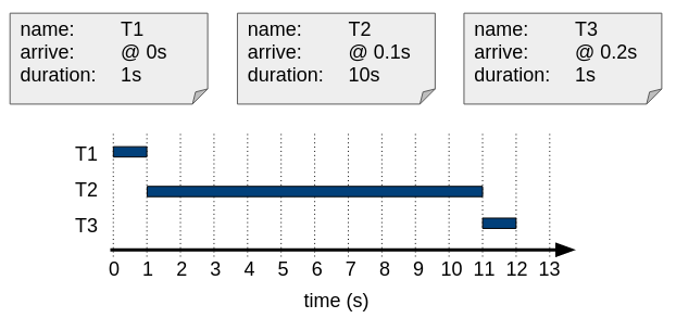
FCFS with cooperative scheduling.
Applying the first three metrics on the example above gives the following results:
Average Throughput:
- 3 jobs over 12 seconds => 0.25 jobs / s
AJWT:
- Task 1 arrives at 0 sec and can immediately start running => wait time: 0s
- Task 2 arrives at 0.1 sec and can start after 1s => wait time: 0.9s => 1s (rounded)
- Task 3 arrives at 0.2 sec and can start after 11s => wait time: 10.8s => 11s (rounded)
- Average Job Wait Time = (0 s + 1 s + 11s)/3 = 12s / 3 = 4s
AJCT:
- Task 1 arrives at 0 sec, waits 0s and takes 1s => duration: 1s
- Task 2 arrives at 0.1 sec, waits 0.9s and takes 10s => duration: 11s (rounded)
- Task 3 arrives at 0.2 sec, waits 10.8s and takes 1s => duration: 12s
- Average Job Completion Time = (1 s + 11 s + 12s)/3 = 24s / 3 = 8s
For these examples, the decimal portion can be rounded away. It is only used to make a distinction in the order of arrival.
SJF
By looking at the FCFS metrics, we can immediately see an easy way to improve the AJWT and AJCT metrics: schedule Task 3 before Task 2!
One algorithm that would allow such an optimization is called Shortest Job First (SJF). With this algorithm the scheduler looks at the tasks that are in the ready state. The shortest job within this queue is allowed first on the processor.
If the scheduler applies the SJF algorithm on the same example, the occupation of the processor looks like shown below.
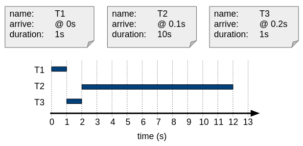
SJF with cooperative scheduling.
Calculate the three metrics for the result of the SJF example, above: Throughput, AJWT, and AJCT.
Throughput = 3 taken / 12 s = 0.25 jobs/s
AJWT = ( 0 s + 1 s + 2 s ) / 3 = 1s
AJCT = ( 1 s + 2 s + 12 s ) / 3 = 5s
We can see that the AJWT and AJCT metrics are indeed improved considerably for this example using SJF!
Preemptive scheduling
Both of the examples for FCFS and SJF have so far been for non-preemptive/cooperative scheduling. Tasks have been allowed to run to their full completion. Let’s now compare this to preemptive scheduling, where the scheduler can pause a task running on the processor. Note that for the practical example we’ve been using, nothing much would change with preemptive scheduling: the selected next job would always be the same (either the first one started that hasn’t finished yet, or the shortest one remaining).
As such, let’s use a slightly more advanced example:
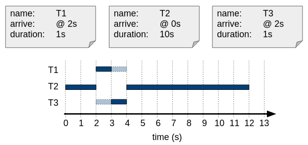
Preemptive scheduling.
For preemptive scheduling, there are again several options to determine when to preempt a running task, as here we’re no longer waiting for a task to end/yield. You could for example switch tasks each x milliseconds/x processor ticks. In our example, the scheduler preempts only when a new job comes in: it stops the currently running job and starts the most recently added job.
In the example above the following actions are taken:
- @ 0s, there is only one job: T2 => schedule T2
- @ 2s, there are two new jobs (T1 and T3) and one old (T2) => schedule T1 (or T3)
- @ 3s, T1 (or T3) is done; there is one old job (T3 (or T1)) and one even older (T2) => schedule T3 (or T1)
- @ 4s, T3 (or T1) has finished; there is one older (T2) => schedule T2
- @ 12s, T2 has finished; there are no more jobs
As such, this example demonstrates a sort-of Last-Come-First-Served (LCFS) approach.
Calculate the three metrics for the result of the preemption example, above: Throughput, AJWT, and AJCT.
Throughput = 3 taken / 12 s = 0.25 taken/s
AJWT = ( 0 s + 0 s + 1 s ) / 3 = 0.33 s
AJCT = ( 1 s + 12 s + 2 s ) / 3 = 5 s
Apply cooperative FCFS and SJF scheduling to the new example tasks and calculate the necessary metrics. Compare the results to the preemptive LCFS.
Priority-based scheduling
At this point we could try a SJF approach with preemption (which here would be called shortest-remaining-time-first). Although this a perfectly fine exercise (wink), in practice estimating the duration of a job is not an easy task, as even the program itself typically doesn’t know how long it will run for! The OS could base itself on earlier runs of the program (or similar programs), or on the length of the program, but it remains guesswork. As such, SJF is rarely used in practice. In our example, it also wouldn’t be the perfect approach, since both T1 and T3 have equal (estimated) durations, and it wouldn’t help the OS to decide which should be run first. Put differently, the scheduler wouldn’t be deterministic.
A more practical approach is priority-based scheduling. In this setup, you can assign a given priority to each task, and have jobs with higher priority run before those of lower priority. This still leaves some uncertainty/non-determinism for processes with the same priority, but it’s a good first approach.
Let’s assume the priorities as mentioned in the image below. Try to complete the graph with the correct scheduler decision.
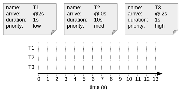
Preemptive scheduling.
As can be seen from the example above, this approach might hold a potential risk: starvation. Some jobs with lower priority (in our case T1) might not get any processor time until all other processes are done: they starve. One solution for starvation is priority ageing. This mechanism allows the priority of a job to increase over time in case of starvation, leading to the job eventually being scheduled. The actual priority thus becomes a function of the original priority and the age of the task. Again, as you can imagine, there are several ways to do this priority ageing (for example at which time intervals to update the priority and by how much, or by how/if you change the priority after the task has been scheduled for its first time slot). We will later see how this is practically approached in Linux.
Round-Robin scheduling
As you can see, scheduling algorithms can get quite complex and it’s not always clear which approach will give the best results for any given job load. As such, it might be easier to just do the simplest preemptive scheduling we can think of: switch between tasks at fixed time intervals in a fixed order (for example ordered by descending Task start time). This is called Round-Robin scheduling (RR).
As such, RR allows multiple tasks to effectively time-share the processor. The smallest amount of time that a job can stay on the processor is called a time quantum or time slice. Typically the duration of a time slice in a modern OS is between 10 and 100 ms. All jobs in the ready queue get assigned a time slice in a circular fashion. An (unrealistic) example with a time slice of 1s is shown below:
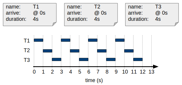
Round Robin scheduling.
Calculate the three metrics for the result of the preemption example, above: Throughput, AJWT, and AJCT.
Throughput = 3 taken / 12 s = 0.25 taken/s
AJWT = ( 0 s + 1 s + 2 s ) / 3 = 1 s
AJCT = ( 10 s + 11 s + 12 s ) / 3 = 11 s
As can be seen from the example above, RR also has some downsides. While each task gets some CPU time very early on (low AJWT), the average completion time (AJCT) is of course very high, as all tasks are interrupted several times. If we were to compute CPU efficiency, this would also be lowest here, due to the high amount of context switches between tasks.
A preemptive scheduler does not wait until a task yields the CPU, but interrupts its execution after a single time slice (or, in previous examples, when a new task arrives).
This does NOT mean however that a task cannot yield the CPU !!!
Another way of putting it is: a job can either run until the time slice has run out (this is when the scheduler interrupts the job) or until the job itself yields the processor. In practice, both of course happen often during normal executing of tasks in an OS.