3.1 Von Neumann Architecture
In order to properly understand some concepts later in this course (such as the C pointers, stack and heap and context switching overhead), it is useful to understand some of the basics of how a CPU works internally and how the OS (and other software) interfaces with it.
The ALU
At its core, a CPU is hardware that enables the execution of a (limited) number of relatively simple/basic mathematical and logical operations. These operations can then be used to construct higher-level fuctionality, eventually leading to full programming language concepts like loops and functions (see later).
A few of these possible operations, applied to one or two parameters (called operands) A and B, are listed below:
| Mathematical | Logical |
|---|---|
| Addition: A + B | A AND B |
| Subtraction: A - B | A OR B |
| Multiplication: A * B | NOT A |
| Division: A / B | A XOR B |
Shift left: A << B |
|
Shift right: A >> B |
|
| Negation: -A |
Most of these operations are typically implemented directly in hardware by a combination of logical ports (AND, OR, NOT, etc.). What that looks like exactly is discussed in your other course Digital and Electronic Circuits (DISCH). For now, the main thing we need to know is that all the operations are typically combined in a single hardware element: the Arithmetic Logical Unit (ALU).
The ALU (wikipedia)
As the single ALU supports multiple operations, we need a way to select which operation is chosen at a given time. This is done using the operation code (opcode), which is really just a number. For example, we can define that number 0 means ADD, 1 means SUB(TRACT), 2 means MUL(TIPLY), etc.
Additionally, the ALU has not one but two outputs: 1) the actual result of the operation, and 2) a number of status signals. One simple example of such a signal is the carry bit, which is used when adding or multiplying binary numbers. This is also why the ALU can receive status signals as input: if the ALU for example works on 32 bits at a time, and we want to add two 64-bit numbers, the carry bit of adding the first two 32-bit parts needs to be passed onto the addition of the second two 32-bit parts. Other signals could for example be if the result was negative, positive, or zero, which helps with comparing two numbers.
Not all possible operations are typically implemented directly in hardware, as they can be reconstructed/created by using other operations in a clever way. For example, negation (-A) can be done by using subtraction (0 - A).
Can you find a clever way of doing the following operations?
- Multiplication by iterative addition
- Multiplication by using shift left (
<<), division by shift right (>>) - Negation by using XOR
- Comparison using subtraction
1. 3 * 5 = 5 + 5 + 5
2. shift left is multiplication by 2 (A * 4 = A << 2), shift right is division by 2 (A / 4 = A >> 2)
3. -A = A XOR 1 (produces ones where zeroes, and vice versa).
4. A - B. If result == 0, A and B are equal. If result < 1, B was larger than A
In practice, full division is difficult to implement directly in hardware and typically uses other operations in a loop, making it a slow operation!
Memory
To function the ALU needs to be passed in the operand values, but it also produces an output value that we probably want to re-use in the future (potentially in the very next calculation!). As such, we need the concept of a memory which stores values (both inputs and outputs). For now, let’s call this the RAM (Random Access Memory), indicating we can access, read and write any part of it at will.
Memory cells are again implemented in hardware by using elements called flip-flops (or similar) and their details are out of scope for this course. It is important however that we need a way to somehow indicate which exact memory cell we want to use at a given time. After all, modern RAM memory can be several GigaBytes (GB) large, and we often only use 32 or 64 bits of that at a time to represent a given number.
To achieve this, most memory assigns a unique number to each group of 8 bits (a single byte) it stores. For example, the first byte in memory is assigned the number 0, the second is number 1, etc. In a 4GB RAM, there are 4,294,967,295 bytes, each of which has its own unique number.
We often call these unique numbers memory addresses (and later in C pointers)! Much like when using the real-life postal system, the address is used to uniquely identify a single byte so we can read/write it.
For example, let’s assume three different byte variables A, B and C are stored in a RAM of 256 bytes. A is at address 3 and has value 15, B is at address 0 and has value 20 and C is at address 1 and has no value yet. The other addresses are empty for now.
The first 8 bytes of the RAM look like this:
| Address | Value | Comment |
|---|---|---|
| 0x00 | 20 | B |
| 0x01 | C | |
| 0x02 | ||
| 0x03 | 15 | A |
| 0x04 | ||
| 0x05 | ||
| 0x06 | ||
| 0x07 |
As such, a simple program performing the operation C = A + B might look like this:
1. Read the value of A from address 3
2. Read the value of B from address 0
3. Pass the value of A and B and the opcode for + to the ALU
4. Write the output value of the operation (20 + 15 = 35) to address 1
The (first part of the) RAM now looks like this:
| Address | Value | Comment |
|---|---|---|
| 0x00 | 20 | B |
| 0x01 | 35 | C |
| 0x02 | ||
| 0x03 | 15 | A |
| 0x04 | ||
| 0x05 | ||
| 0x06 | ||
| 0x07 |
Instructions
Now you might wonder: but how do we actually know we need to read A and B, perform the + and write to C? We don’t just need a way to store the operand values, we also somehow need to store the operation itself!
The way we do this is typically called an instruction, which specifies not just the operation we want the ALU to perform (+) but also on which values to perform it and where to put the output. For the example above, the instruction would have to encode the following four parameters to be useful:
instruction type, address of first operand, address of second operand, address of output
Crucially, each of these four parameters can just be represented as a number!
In the original computers, these values would often be hardcoded into hardware (fixed/single program) or be set manually, for example using buttons and knobs (you can imagine how slow that was…). Later computers would use so-called punch cards: thick papers with holes punched in specific locations to indicate a binary 1 or 0 value to make up the numbers.
Later however, several scientists (Johh von Neumann and others) had a revolutionary idea: since instructions can be represented as numbers, just like the data they operate upon, instructions can be stored in the same memory used to store the data! This way, we can very easily write computers that can run arbitrary programs efficiently: just change the instructions in the memory!
The above example C = A + B could then look something like this:
| Address | Value | Comment |
|---|---|---|
| 0x00 | 20 | B |
| 0x01 | C | |
| 0x02 | ||
| 0x03 | 15 | A |
| 0x04 | ||
| 0x05 | ||
| 0x06 | ||
| 0x07 |
| Address | Value | Comment |
|---|---|---|
| 0x08 | 0 | ADD instr. type |
| 0x09 | 0x03 | A address |
| 0x0A | 0x00 | B address |
| 0x0B | 0x01 | output address |
| 0x0C | ||
| 0x0D | ||
| 0x0E | ||
| 0x0F |
Note: here we represent addresses as hexadecimal values and non-addresses as decimal numbers. This is just for convenience and by convention, not because it’s really needed!
We see that we’ve split a single instruction over 4 different bytes in memory. Conceptually, we could have tried to encode it all in a single byte as well, for example by taking the first 2 bits as an opcode, the next 2 bits as address 1, another 2 for address 2, etc. However, as you can see, that would severly limit the amount of values we could represent (2 bits can only mean 4 options (0, 1, 2, or 3) and so only 4 opcodes or 4 memory addressess…). By using more memory for each, we allow a wider range of values.
Note that 8 bits (1 byte) for an address is still very little (only allows us to address 256 bytes). Real instruction encodings typically either use more than 1 byte to represent an address or use multiple steps to load a full address (for example for a 32-bit address, first load one 16-bit part with 1 instruction, then the second 16-bit part with another instruction). Other clever tricks are used, such as using an offset from a starting address (for example when storing an array), so you don’t always need to create larger addresses. This is however not important for this course yet. Here we can just assume a simple 256-byte RAM where all addresses fit nicely into a single byte!
This concept of the “stored program” might seem trivial to you today (after all it’s how all modern computers work), but it was quite revolutionary at the time!
Up until now we’ve only discussed a very simple program with just one instruction. Let’s think about what happens if we have a slightly more complex program:
C = A + B
E = C - D
Show what the first 16 bytes of the RAM might look like after executing this program if we encode the second instruction right after the first (so starting at address 0x0C), if D has the value 10 and if the - operation has an opcode of 3.
You can choose yourself where to store D and E.
| Address | Value | Comment |
|---|---|---|
| 0x00 | 20 | B |
| 0x01 | 35 | C |
| 0x02 | 10 | D |
| 0x03 | 15 | A |
| 0x04 | 25 | E |
| 0x05 | ||
| 0x06 | ||
| 0x07 |
| Address | Value | Comment |
|---|---|---|
| 0x08 | 0 | ADD instr. type |
| 0x09 | 0x03 | A address |
| 0x0A | 0x00 | B address |
| 0x0B | 0x01 | C address |
| 0x0C | 3 | SUB instr. type |
| 0x0D | 0x01 | C address |
| 0x0E | 0x02 | D address |
| 0x0F | 0x04 | E address |
Immediates
Up until now we’ve assumed that all the initial values we’ve used (say 15 for A and 20 for B) are somehow already present in memory. But how do they actually get there in the first place?
You might think of a scheme were you put every possible number somewhere in memory at boot time and then just read the necessary address if you need a fixed number. However, that would be quite inefficient!
Instead, we can define some new instruction variants that don’t work on addresses, but on numbers instead:
-
Previous format: all addresses: for C = A + B
instruction type, address of first operand, address of second operand, address of output -
New format 1: all constants: for C = 12 + 33
instruction type, constant value, constant value, address of output -
New format 2: one address and one constant: for C = A + 33
instruction type, address of first operand, constant value, address of output
This means that our basic operations have 3 versions each, so we should also have different names:
- no suffix: 2 addresses (ex. ADD)
- d suffix (direct): 2 immediates (ex. ADDd)
- i suffix (immediate): 1 address, 1 immediate (ex. ADDi)
Now you can also see why the instruction number for SUB was 3 instead of 1 above! We were reserving room for extra ADD instruction variants. Now, we can say that ADD = 0, ADDd = 1, ADDi = 2, SUB = 3, SUBd = 4, and SUBi = 5;
We use the term immediate here for constant values that are directly encoded into an instruction, because that’s what they’re typically called in real Assembly languages. Put differently: this value is “immediately available” once we’ve read the instruction from memory; we don’t have to fetch another value from an address to be able to use it. This is because addresses are just numbers in memory, and so they can also be replaced with other numbers!
With this we can re-write the previous example so it does not rely on values already being in memory before starting:
C = 15 + 20
E = C - 10
| Address | Value | Comment |
|---|---|---|
| 0x00 | ||
| 0x01 | 35 | C |
| 0x02 | ||
| 0x03 | ||
| 0x04 | 25 | E |
| 0x05 | ||
| 0x06 | ||
| 0x07 |
| Address | Value | Comment |
|---|---|---|
| 0x08 | 1 | ADDd instr. type |
| 0x09 | 15 | immediate value |
| 0x0A | 20 | immediate value |
| 0x0B | 0x01 | C address |
| 0x0C | 5 | SUBi instr. type |
| 0x0D | 0x01 | C address |
| 0x0E | 10 | immediate value |
| 0x0F | 0x04 | E address |
Note that we no longer need a separate memory address for A, B or D, as their values are now encoded into the instructions themselves (see address 0x09, 0x0A and 0x0E)!
How would you load a hardcoded value into a memory address, using only the instructions seen so far? For example: int X = 50; where X is at address 0x07?
ADDd 0 50 0x07
Branching and the Program Counter
For now, we’ve assumed that instructions that are sequential in memory also get executed one-by-one. Additionally, we’ve assumed we always start execution at address 0x08 (as our first instruction has always been there). However, this is of course not always the case, nor something we always want.
A simple example would be the following C (pseudo)code:
int C = A + 10;
if ( C != 20 ) {
   C = 0;
}
int D = C - 10;
In this case, we see that we can’t just encode the instructions in sequence and execute them one-by-one, as that would always do the C = 0 operation! As such, we need a way to skip one or more lines if a certain condition is true (in this case if C == 20).
For this reason, we will introduce the concept of a Program Counter (PC). This PC keeps track of which instruction we’re executing at any given time. Since our instructions are really just numbers in our RAM memory, the PC really just contains an address pointing to an instruction!
Let’s use our original example without the if-test. In these cases, the PC started at a value of 0x08, executed the instruction there, and was then incremented by 4 to 0x0C, the start of the next instruction. Note that it’s incremented by 4 instead of just 1, because each instruction is spread over 4 bytes!!! As such, usually we can just do PC = PC + 4 after each instruction and the program will run as intended.
Written out, this is what happens with the PC during the simple program’s execution:
- initialize the PC at address 0x08
- load the instruction at 0x08 (and the three bytes after that)
- execute the instruction (C = A + B)
- PC = PC + 4. New value is 0x0C
- load the instruction at 0x0C (and the three bytes after that)
- execute the instruction (E = C - D)
- PC = PC + 4. New value is 0x10
- there is nothing at 0x10, the execution stops
However, once we encounter an if-test, we need a way to change the PC to another value. In our example, the ADDi is at address 0x08, and it is executed normally. Then, the instruction for the if-test (see below) is at 0x0C. If C == 20, then we want to skip the next instruction at PC + 4 (at 0x10, which is C = 0) and instead go to the one beneath the if-test at PC + 8 (at 0x14, D = C - 10). So we want to do either PC = PC + 8, or maybe better: PC = 0x14, instead of the normal PC = PC + 4.
| Address | Value | Comment |
|---|---|---|
| 0x00 | 10 | A |
| 0x01 | ||
| 0x02 | C | |
| 0x03 | D | |
| 0x04 | ||
| 0x05 | ||
| 0x06 | ||
| 0x07 |
| Address | Value | Comment |
|---|---|---|
| 0x08 | 2 | ADDi instr. type |
| 0x09 | 0x00 | A address |
| 0x0A | 10 | immediate value |
| 0x0B | 0x01 | C address |
| 0x0C | 13 | BEQi instr. type |
| 0x0D | 0x01 | C address |
| 0x0E | 20 | immediate value |
| 0x0F | 0x14 | branch address |
| Address | Value | Comment |
|---|---|---|
| 0x10 | 3 | ADDd instr. type |
| 0x11 | 0 | immediate value |
| 0x12 | 0 | immediate value |
| 0x13 | 0x01 | C address |
| 0x14 | 5 | SUBi instr. type |
| 0x15 | 0x01 | C address |
| 0x16 | 10 | immediate value |
| 0x17 | 0x03 | D address |
As such, you see we have created a “split” in the way the program can execute: it can always take just 1 of 2 paths, not both at the same time (either we skip 0x10 or not)! This is often compared to a tree branch, which splits off into several smaller branches and you can only follow one. Hence, in (low-level) programming, an if-test is often called a branch.
It should be no surprise then that the instruction to represent our if-test is called BEQ (Branch if EQual). This one is a bit different from the previous ones, since it doesn’t have a real “output” address. Instead, it has an address (0x14) that the PC should be set to if the condition (C == 20) is true. If the condition is NOT true, nothing special happens (the BEQ does “nothing”) and the PC is just increased by 4 as usual.
Written out, this is what happens with the PC during the if-test program’s execution if A was 10 at the start:
- initialize the PC at address 0x08
- load the instruction at 0x08 (and the three bytes after that)
- execute the instruction (C = A + 10)
- PC = PC + 4. New value is 0x0C
- load the instruction at 0x0C (and the three bytes after that)
- execute the instruction ( C == 20? )
- after the last instruction, the value at adress 0x01 (C) is indeed 20, so we want to manually set the PC
- PC = third byte of the current instruction = 0x14
- load the instruction at 0x14 (and the three bytes after that)
- execute the instruction (D = C - 10)
- PC = PC + 4. New value is 0x18
- there is nothing at 0x18, the execution stops
Note that we here have just two variants: BEQ with 2 addresses and BEQi with an address and an immediate, as BEQd wouldn’t be very useful in a real programme (can you explain why?). The two variants look like this:
BEQ : instruction type, address of first operand, address of second operand, address to set the PC to if condition is true
BEQi: instruction type, address of first operand, constant value, address to set the PC to if condition is true
Note also that we use inverse logic to the C pseudocode. There, the if-test is C != 20, while here we use BEQ to test C == 20 if we want to SKIP the contents of the if-test. As you can imagine, there are also the BNE (Branch if Not Equal) and BNEi instructions that do the opposite logic. Other similar instructions are BLT (Branch if Less Than) and BLE (Branch if Less than or Equal). Commonly, most CPUs don’t have BGT or BGE instructions (can you explain why?).
Note that we’ve now seen many examples where the instruction type does not map directly to the ALU opcode. For example, the BEQ instruction internally probably uses a SUB to compare two values (remember from before, if A - B == 0, they were equal). As such, the CPU internally often needs to “decode” an instruction and perform some extra steps (map instruction type to an ALU opcode, fetch values from memory if they’re not immediates) before actually executing it.
We’ve now been using two different notations interchangeably. On one hand, we have C = A + B and on the other we have ADD A B C (which is the way the instruction is encoded in the RAM). While we’re most used to the first, the latter is typically how low-level “Assembly” code is written.
As such, our program
int C = A + 10;
if ( C != 20 ) {
   C = 0;
}
int D = C - 10;
Can also be written as:
ADDi A 10 C
BEQi C 20 0x14
ADDd 0 0 C
SUBi C 10 D
For a real-life example, you can execute the following command objdump -d /bin/bash | head -n 30, which shows you the first 30 lines of x86 assembly of the bash program. This assembly is quite a bit more advanced than our dummy examples and uses some different names, but the concepts are the same!
Jumping
By now, you might have noticed that our branching instructions won’t be enough to represent even slighty more complex programs such as the following if-else. With our current understanding of Assembly we don’t really know what to do with the else, so this would translate to:
int C = A + 10;
if ( C != 20 ) {
   C = 0;
}
else { // if C == 20
    C = 50;
}
int D = C - 10;
0x08: ADDi A 10 C
0x0C: BEQi C 20 0x14 // the if test, jumps to the else body if equal
0x10: ADDd 0 0 C  // body of the if

// I don't know the instruction for an "else" yet, so just do nothing?
0x14: ADDd 0 50 C // body of the else

0x18: SUBi C 10 D
If we would implement this as before, where the BEQi is essentially ignored if C != 20, this would first execute C = 0 and then ALSO the C = 50 (the else body).
You can see we really need to skip not just 1 line if C == 20 as before, but now we also need to skip a line if C != 20! In the latter case, we need to skip the C = 50. The naive way of doing this would be to just add the opposite branch instruction before the else:
0x08: ADDi A 10 C
0x0C: BEQi C 20 0x14 // the if test, jumps to the else if equal
0x10: ADDd 0 0 C  // body of the if

0x14: BNEi C 20 0x1C // the else, jumps to the end if not equal
0x18: ADDd 0 50 C // body of the else

0x1C: SUBi C 10 D
int C = A + 10;
if ( C != 20 ) {
   C = 0;
}
if ( C == 20 ) {
    C = 50;
}
int D = C - 10;
You can see this approach is equivalent to changing the else to an if (C == 20) in C. This works, but really only in this particular case. Let’s think about what happens if the body of the if-test would look a little different, and instead of C = 0 it would do C = 20:
int C = A + 10;
if ( C != 20 ) {
   C = 20;
}
if ( C == 20 ) {
    C = 50;
}
int D = C - 10;
int C = A + 10;
if ( C != 20 ) {
   C = 20;
}
else {
    C = 50;
}
int D = C - 10;
With our approach on the left, we would ALSO execute the “else” (which is now the second if-test C == 20), while with the original code on the right, it would properly skip the else.
We can see that, ideally, we would have another way of specifying the else without having to repeat the original condition somehow (C != 20). What we really want is to just skip the else block entirely if the if is taken. Put differently, at the end if the if-block, we want to change the PC so that it goes to the instruction right after the else! This is something we always want to do for that if (we always want to skip the else) and thus we don’t really need to have a condition: it just needs to happen every time.
For these situations (change the PC every time, not just if a condition is true), we can use the JMPi (Jump immediate) instruction. If a JMPi is executed, it just sets the PC to the specified value, no questions asked! As such, the JMPi is about the simplest instruction we’ve seen yet:
JMPi: instruction type, address to set the PC to
With the JMPi, our code remains simple to write but now also executes correctly:
int C = A + 10;
if ( C != 20 ) {
   C = 20;
}
else { // if C == 20
    C = 50;
}
int D = C - 10;
0x08: ADDi A 10 C
0x0C: BEQi C 20 0x18 // the if test, jumps to the else body if equal
0x10: ADDd 0 20 C  // body of the if
0x14: JMPi 0x1C    // always skip the else if the if was executed

0x18: ADDd 0 50 C  // body of the else

0x1C: SUBi C 10 D
Note: the JMPi is conceptually part of the if-block, not the else block. The else really is just the code inside. It is the end of the if-block that jumps OVER the else code if it was executed!
Note that there of course also exists a JMP instruction. However, that one doesn’t just encode the new value for the PC directly. Instead, it encodes an address in memory. To get the new value for the PC, we need to load the value of that memory address, which itself is also an address, and then set the PC to that value, not the immediate encoded in the instruction itself.
This idea that an address can point to a value that is itself another address that can point to another thing is a very powerful concept in C/C++ that allows many fancy features. In the next part, we’ll see how we can use it to implement function calls. For now however, we’ll just use the JMPi variant.
Note finally, for completeness, that “real” Assembly typically does not work with full addresses but “offsets”. For example if the PC is currently at 0x10 and we want to JMPi to 0x18, we wouldn’t say 0x18, but rather 8, because the current value (0x10) plus that offset (8) equals the target address 0x18. Can you guess why this is the common approach?
Clock
A final aspect that is needed to make this all work is called the CPU Clock. This is a timer that runs at a given frequency (say 2-4GHz in modern processors). Each “tick” of the timer means a single instruction can be executed. Put differently: each tick the program counter is changed (either it is incremented by 4 automatically, or moved to a different address by an instruction like BEQ or JMPi).
As such, for a 2 GHz processor, it could execute up to 2 billion (2.000.000.000!!!) instructions per second. You can see that modern CPUs really are crazy fast.
However, in real systems there are challenges that prevent real CPUs from always reaching their full potential (pipeline stalls, data and control hazards, branch prediction errors, port contention, etc.). These aspects are discussed in later courses like “Computer Architectures” and “Software Engineering for Integrated Systems”.
Von Neumann Architecture
The system and its instructions we’ve discussed form the basis of what’s called a Von Neumann architecture. As said before, this is named after John Von Neumann, who was one of the first to describe such as system.
Adapted from wikipedia, a possible (partial) definition for a Von Neumann system is “a design architecture for an electronic digital computer with these components:
- A processing unit that contains an arithmetic logic unit (ALU)
- A control unit that contains a program counter (PC)
- Memory that stores both data and instructions
- External mass storage
- Input and output mechanisms
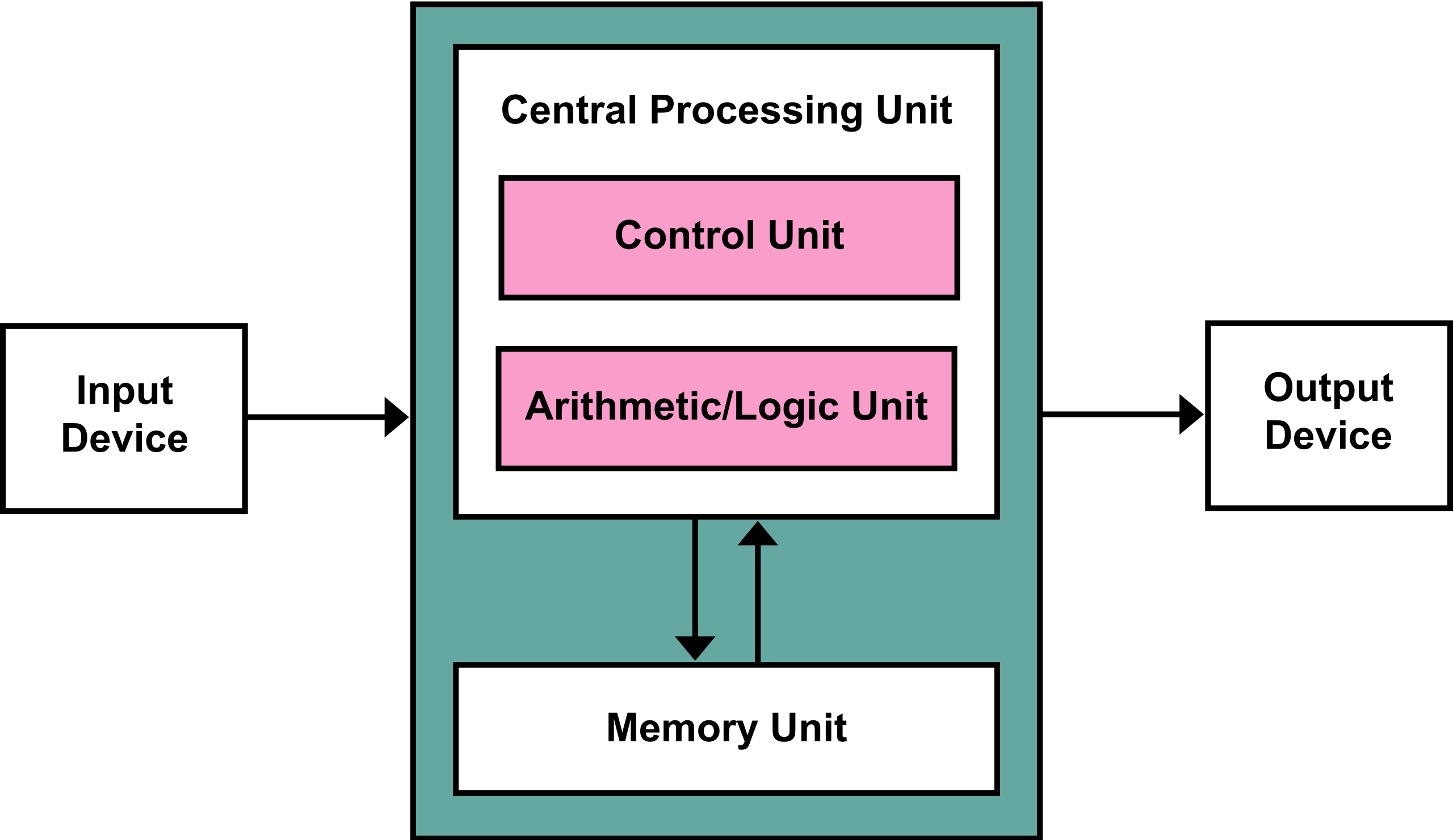
The high-level Von Neumann architecture (source: wikipedia)
A final note on safety
Note again that in a Von Neumann architecture, both data and instructions are stored in memory. Additionally, there are instructions that can write/manipulate what’s in that memory.
Consequently, you could think of a hacker that writes code that has the goal to overwrite/change other, existing code, and make it do bad/wrong things! For example, a hacker could overwrite the target address of a JMPi instruction (just place a new number at the correct address in memory) and make the else of an if-else execute their code instead of the “real” code!
For this reason, there are often strict separations in place between memory that stores instructions and memory that stores data (we will call them “segments” later in this course). Furthermore, instruction memory is often read-only, except in a few very special circumstances, in which there are other safety measures put in place.
Finally, program A typically cannot access the memory of program B at all! This is one of the core responsibilities of the operating system: to make sure programs cannot access each other’s memory. Not just so they can’t read each others data, but as we’ve now seen, also so they can’t change each other’s instructions! There are exceptions to the rule, such as shared memory models, which will be explained in chapter 6: inter process communication.