7.3: Towards real-world schedulers
The previously discussed scheduling algorithms are but a select number of a huge amount of imaginable approaches that can be thought of. We have seen that all individual algorithms come with certain challenges/downsides that make them difficult for direct use in real-world scenarios. And we haven’t even taken into account all variables that are in play in a typical OS!
As such, in this Section, we first look at a few factors that come into play in real systems. We then look at how the naive schedulers we’ve already seen can be adapted to deal with these new problems. Finally, we discuss how all of this has been combined in practice in the Linux OS scheduler over time.
Reponsiveness vs Efficiency
In theory, we could say that using a Round-Robin (RR) scheduler would be a good starting point. After all, this is a very fair scheduler that ensures that all processes get at least some time on the CPU (so there is no starvation as with a pure priority-based scheduler).
In this section, let’s start from a simple RR scheduler and discuss why it’s difficult to make it work properly in a real-world setting. This is mainly due to three factors:
- Context switching overhead: this limits how often we can switch between tasks
- I/O vs CPU-bound processes: this means we can’t use a single time slice length for all tasks
- Need for priorities: while pure priorities aren’t optimal, we still want to use their concept to be able to speed up certain key tasks
Context Switching Overhead
As said previously, when a new task is scheduled for execution by the OS, a number of operations need to happen to swap the old task with the new one. In the previous examples, we’ve pretended these operations happen instantly (the context switching overhead was 0), but that’s of course not the case.
Say we have 2 user tasks: X and Y. X has already been running for a while on the processor, while Y is in the ready state, waiting for CPU-time. After X’s time slice is up, the OS uses the RR scheduler to select Y as the next task to run. Switching between the tasks involves the following steps:
-
Step 1
X has be stopped in such a way that it can continue from where it left off the next time it is scheduled. Therefore, a snapshot has to be made: what is the value of the program counter, what are the values in the registers, which address is the stack pointer pointing to, what are the open files, which parts of the heap are filled, … ? All these values need to be stored. As was discussed in Chapter 6, the OS keeps a PCB (Process Control Block) for every process, which contains the fields necessary to store all these required parameters: The PCB of X needs to be updated to the current CPU. The kernel then puts this PCB in a list of paused tasks.
Note: something similar happens for Threads (remember there’s also a conceptual TCB), but it’s more lightweight, since there is more shared state between threads in the same program and so fewer aspects need to be updated.
-
Step 2
X is removed from the processor. For example, the register contents and program counter are cleared.
-
Step 3
The scheduler uses the RR scheduling algorithm to determine which process is next. Since Y is the only other process, it is selected. The processor searches Y’s PCB in its list of paused tasks.
-
Step 4
Everything that happened to the PCB of X, now needs to be done in the opposite direction with the PCB of Y: the PCB of Y needs to be restored. The program counter is read and the next instruction is loaded. The values of the registers are restored. The stack pointer is updated.
-
Step 5
Y starts to run on the processor.
In the previous Section, we have called this series of actions “Dispatching”. As such, the time it takes for the dispatcher to stop one process and start another running is known as the dispatch latency, or the scheduling latency. The actions of updating (and restoring) individual PCB’s is typically referred to as a context switch (though some sources also call the entire process together a context switch).
As you can see, during the dispatch period, the CPU is not actually doing any useful work: it is waiting and/or updating its state so the new task can start running. As such, the act of dispatching a new process is considered 100% overhead, and it should be avoided as much as possible. Note: there are also other aspects that make context switches slower, such as the fact that it often means that data in the cache memory is no longer useful. As the cached data belongs to the previous task, the cache needs to be (partially) flushed and updated with data from the new task as well, which again takes time.
However, before you get the wrong idea, it’s not all that bad. In practice, the dispatch latency is typically in the order of (10) microseconds (say about 1/100th of a millisecond). Still, if we were to switch processes for example each millisecond, we would have a full 1% overhead, which over time definitely adds up (we don’t only spend more time context switching, we also do a larger amount of context switches over time). If you recall from the previous section, we introduced the metric CPU efficiency (ηCPU), which helps make concrete how much overhead actually was introduced.
We can see that we somehow need to strike a balance between being CPU efficiency (less overhead) and keeping the system responsive (switching between tasks often enough). This is easy enough in our simple examples with just 3-10 tasks, but modern systems often run hundreds of tasks at the same time.
The length of the RR time slice thus plays a large part in this: shorter time slices make things more responsive, but cause more context switches, and vice versa. As such, we want to determine an ideal time slice length, but it’s not easy to see how this can be accomplished. In general, we can really only say that the time slice should always be quite a bit larger than the dispatch latency, but that we don’t really have an easy way to determine an upper bound.
I/O-bound vs CPU-bound tasks
A second aspect that’s highly relevant in modern systems is that there are typically two large classes of tasks: I/O-bound and CPU-bound tasks.
-
The I/O-bound tasks typically run for only short amounts of time (a few milliseconds) before they already have to wait for an I/O operation. Put differently, these tasks often pause themselves (go into the “waiting” state) often. A good example is a program that’s listening for user input (keyboard/mouse). These tasks are thus sometimes also referred to as interactive tasks. However, waiting for packets to come in from the network is also an I/O operation, as is for example waiting for a large file to be loaded from hard disk into RAM memory so it can be used. More generally, an I/O bound task is a process that can’t execute (many) useful instructions on the CPU (at this time) because it doesn’t have the necessary data/input available (yet).
-
The CPU-bound tasks typically do not require much outside input and/or mainly have to run a lot of calculations on the data. As such, if the data is available, these tasks can keep issueing instructions to the CPU for a long time without pause. They run for tens of milliseconds (or much more) without ever yielding/waiting themselves. These jobs typically process data in large chunks, and are sometimes called batch tasks.
The fact that there are typically few processes that do “something in between” (few programs can do a medium amount of calculations with a medium amount of data) again makes it difficult to determine a good time slice length:
-
If there are many I/O-bound tasks, shorter timeslices are probably better, as most tasks will pause themselves frequently anyway, and we don’t loose much (extra) efficiency for higher responsiveness.
-
On the other hand, if there are many CPU-bound tasks, longer timeslices are probably better, as processes will typically fill their slices with useful work and we reduce the amount of context switches (and those tasks typically don’t need to be very responsive).
Note that many processes switch between being I/O-bound and CPU-bound over the course of their execution. Take for example Photoshop: here, you often want to first load a (very) large image file into RAM memory from disk (or network nowadays) to then use advanced image processing tools on it (e.g., apply a sepia filter).
As such, while waiting for the image data to become available on the CPU, Photoshop is I/O bound and can’t do much. However, once the data is available, it will want to execute heavy calculations on it, causing it to become CPU-bound for the duration of the calculations.
Simply using an average time slice that’s “somewhere in between” can produce the worst of both worlds: it lowers the responsiveness in interactive systems (as batch processes delay interactive processes), while (needlessly) increasing the amount of context switches during batch processing.
As in the previous subsection, it’s unclear how long a time slice should ideally be to deal with both I/O and CPU-bound tasks, and especially with tasks (like Photoshop) that can switch from one category to the other, depending on what they’re doing at a given time.
Singular time slice length example
Let’s illustrate this with an example:
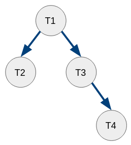
- There are two I/O-bound tasks, T1 and T2. Both run for 1ms, in which they update state, and then wait/yield for more input.
- Input becomes available after 4ms of wait time (starts when the task yields). The task then becomes “ready” to process this input.
- Both tasks do three rounds of this (wait for input 3 times in total)
- There is one CPU-bound task, T3, that runs a total of 10ms without yielding
- All three tasks start/arrive at 0s and input is available for T1 and T2 at 0s
- The two I/O-bound tasks are higher priority than the CPU-bound task.
- Each task gets to complete its full time slice unless it yields by itself.
- In this very unrealistic system, the dispatch latency is a full 1ms
Draw schemas of how these tasks would be scheduled in two scenarios:
- with a time slice of 2ms
- with a time slice of 5ms.
Indicate clearly each time a task goes into a ready state and don’t forget to take into account the high dispatch latency!
For each scenario, calculate the CPU efficiency ηCPU (the percentage of time that the processor performs actual work: total runtime - dispatch latency overhead). Note that calculating AJWT is less useful here to compare both scenarios, as we have multiple waiting periods! As such, focus on the AJCT and calculate that for the three tasks as well.
Answer these questions:
- How many context switches are there in each scenario?
- Which scenario is more efficient? Why?
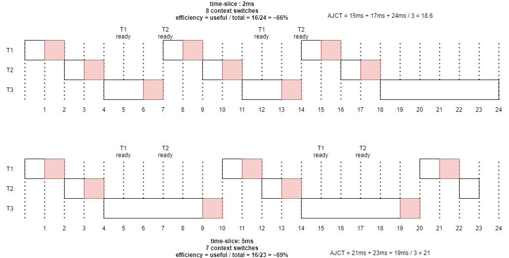
Comparison between two time slices
Dynamic Time Slice Length
As we can see from the example above and the discussion before that, it’s indeed difficult to find an optimal, singular time slice length for all processes in a system over time.
However, there is a relatively simple insight that we should get by now: if the optimal time slice depends on how often the processes pauses itself (which is often for I/O-bound, and more rare for CPU-bound), we can start assigning dynamic time slice lengths to processes, depending on their past behaviour!
For example, if task X got a time slice of 20ms, but paused itself after just 5ms, we might decide to give it just a 10ms time slice the next time it’s scheduled, as we expect it to be I/O-bound. Inversely, if task Y does run for its complete 20ms time slice, we might increase that to 30ms the next time, as it’s probably CPU-bound.
Note that, even if a task evolves from I/O bound to CPU-bound (or back), the logic still works! The time slice will keep adjusting itself dynamically over time to accomodate whatever a task needs at a given time.
This is a very elegant yet powerful solution that is indeed used in practice. However, it also has some challenges. Two of the main ones are:
- We still need lower and upper bounds for the time slice lengths, which are not trivial to determine
- CPU-bound tasks can still end up blocking I/O-bound or interactive tasks, especially if the CPU-bound tasks get a relatively large time slice!
This latter point isn’t a problem if the CPU-bound task is something the user is actually waiting for (e.g., using Photoshop). However, if it’s a background process that’s processing data (for example updating a search index, scanning files for viruses), we would rather not have that process interupting more important tasks (e.g., while the user is using a Web browser).
As such, even with dynamic time slice lengths, we still need to add the concept of priorities of processes, to make sure we can manually (using C APIs, see the lab in 7.4) or automatically (e.g., which window is the user currently interacting with) ensure important processes are given more CPU time.
Priorities
As discussed in the previous section, we often want to explicitly indicate a given task is more important than another. This is usually done using priorities, whereby each task is assigned a number so they can be fully ordered to determine which is most important.
In the simple Priority-based scheduler we’ve considered, the priority was mainly used to determine when to start which process, as higher priority processes are selected earlier. However, we’ve also seen that this could lead to starvation for low-priority tasks, needing some ageing mechanism (whereby the priority is slowly increased for low-priority tasks over time) to correct this.
Applying this idea that priorities influence when a task is scheduled to our preemptive RR scheduler with dynamice time slices, we see it becomes more like an how often is a task to be scheduled! For example, higher priority tasks can be scheduled more often than/before lower priority tasks, independent of their (dynamic) time slice length. While that works conceptually, it does not really help prevent starvation.
However, can we not think of another, quite different, way to interpret priorities rather than when a task is scheduled?
Imagine for a second that, rather than controlling the timing of when a task is scheduled, instead we use the priority (rather than how often a task pauses itself) to determine the per-process time slice length.
For example, high priority jobs could get a longer time slice (say 10ms) to make sure they get to do as much work as possible, while lower priority tasks could get less time (say 2ms per burst). We can then use the simple RR scheduler between the different tasks, as the priorities are enforced by the time slice length, rather than by strict execution order/scheduling time. Lower priority processes would get time on the CPU more often than with a direct priority-based scheduler, but in shorter bursts, solving ageing while keeping relative priorities intact.
This seems like a good idea, but we can again question if this will work well in practice. For example, say the high priority tasks in a system are I/O-bound and the low priority tasks are CPU-bound, the proposed system seems to do the exact opposite of what we want (as I/O-bound tasks don’t need long time slices, but batch jobs do).
As such, we now have two competing ways to determine our dynamic time slice length:
- Based on how often a task pauses itself / how often it uses its entire current time slice
- Based on the task’s priority
It is difficult to know which of both is optimal for any given use case, and as you might predict, in practice a combination of both is used (see the Linux schedulers below). This also still doesn’t solve our lower/upper bound for time slice lengths.
A dynamic solution
To summarize our discussion so far: at this point it’s clear that we have multiple different requirements of a real world scheduler: it needs to be both responsive and CPU efficient, it needs to support both I/O-bound and CPU-bound tasks in a decent way, and it needs to have support for per-task priorities to allow further tweaking of scheduling logic.
As we’ve seen, the concept of a Round-Robin scheduler using dynamic time slice lengths is a promising solution, but we’re still not sure how to properly choose the time slice lengths… If we were to think about this further, we would end up at the conclusion that there is no single optimal answer and we will have to use combinations of different options to reach good results.
The general concept of such a solution that combines multiple options is the multi-level feedback queue scheduler. In this setup, we no longer have a single long list of processes, but instead distribute them across multiple, independent “run queues”. Each of these queues can then employ their own scheduling logic (for example use FCFS or RR or even priority-based) and determine other parameters such as if the queue is processed cooperatively or preemptively (in which case, the time slice length can also vary). That’s the “multi-level” part.
The “feedback” part indicates that tasks can move between these separate queues over time (for example as they become more or less important (change priority), as they run for longer or shorter bursts, etc.).
We can then see that we also need a sort of top-level scheduler, that determines how the different run queues are processed (for example, queue 2 can only start if queue 1 is empty if we use FCFS between the queues).
One of the first examples of this approach was given by Fernando J. Corbató et al. in 1962. Their setup has three specific goals:
- Give preference to short jobs.
- Give preference to I/O-bound tasks.
- Separate processes into categories based on their need for the processor.
To achieve these goals, they employ three differen run queues:
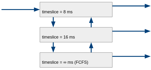
When a newly created process is added to the scheduler, it arrives at the back of the top queue (8ms). When it is scheduled, there are two options: (a) either it runs the full 8ms or (b) it yields before that. In the case of (b), it’s likely that we have a short and/or I/O bound task. As such, when it is done waiting, it is appended at the back of the top queue again.
In the case of (a) however, it’s more likely that we have a CPU-bound task. As such, after the 8ms, it is pre-empted and we move it down to the middle queue (16ms), where it should get a longer time slice next time it is run. We can see this improves efficiency, as we can assume the task will remain CPU-bound and thus we have only half the context switches for these processes!
If the processes in the middle queue keep running to their full time slice of 16ms multiple times, this is an indication they are very heavily CPU-bound. In response, we move them down to the bottom queue. Here, processes are run in FCFS fashion until completion.
Finally, processes can move up to the previous queue if they yield to an I/O operation. This allows for example mostly batch tasks to still get a bit more execution time if they have phases in their programming that requires some I/O work.
Across the three different run queues, a simple FCFS logic is applied: the top queue is processed until it is empty and only then are tasks from the middle queue scheduled. Note: if I/O bound tasks are waiting, they are of course no longer in the top queue, otherwise the bottom queues would never get any time! Only tasks ready to execute are in the queues.
As said in the previous Section, it is difficult to do Shortest Job First (SJF) scheduling, since it’s difficult to know the total duration of a job. This type of setup however tries to approximate this logic by looking not at the total duration of a job, but at the duration of individual “bursts”. Longer jobs automatically move down to the lower queues, leaving more room for jobs with shorter bursts at the top.
The setup described above is of course highly specific to those three goals and needs of a particular system. The concepts of the multi-level feedback queue are however much more flexible, as we can also envision other ways of partioning queues to model other advanced scheduling setups. For example:
- Each level can represent a separate priority (doing for example RR within each level gives us the simple Priority-based scheduler from the previous Section)
- Each level can represent a separate scheduler (the first level can for example do RR, the next FCFS, the next priority-based, etc.)
- Each level can represent a different time slice length (the first has slices of 8ms, the next 16ms, etc.)
Between the levels, we can then also employ other schedulers than FCFS of course (e.g., a RR scheduler, a priority-based scheduler etc.) to improve the responsiveness of tasks in the lower levels.
In practice, these aspects are often combined in specific ways to get a desired outcome (as with the example above). This outcome depends on the system and intended usage. We will see several options for this in the next Section on Linux schedulers. In some way, most modern OS schedulers are variations on the general multi-level feedback queue scheduling concept.
Linux Schedulers
Now that we’ve explored some of the practical issues with real-world scheduling and introduced a basic solution framework, it’s time to look at how things are practically done in the Linux OS. This again goes one step beyond the scheduling logic, as we now need to also take into account performance of the implementations and datastructures, as well as the provided API for programmers (for example, how to actually manipulate priorities in practice).
Over time, the Linux kernel has used different schedulers, of which we will discuss three here. Linux kernels with version 2.4 - 2.6 (before 2003) were using the O(n) scheduler, in 2.6 - 2.6.11 (2003-2007) the used scheduler was O(1), and from 2.6.12 (after 2007) onward the Completely Fair Scheduler (CFS) is mainly used. These schedulers are briefly touched upon here. All of these are preemptive schedulers that incorporate priorities, but as we will see, they do this in various different ways.
You might be confused by O(n) and O(1). This “Big Oh” notation is an often used concept in computer science to indicate the worst-case performance (called “time complexity”) of a program. In general, the factor inside of the O() function should be as small as possible. As such O(1) is optimal (“constant time”), while O(n) indicates that in the worst-case, the program scales linearly with (in this case) the amount of tasks (n). Exponential setups like O(n*n) and especially O(2^n) are to be avoided. In practice, O(log N) is often the best you can do.
O(n) scheduler
The O(n) scheduler got his name from the fact that choosing a new task has linear complexity. This is because this scheduler uses a single linked list to store all the tasks. Upon each context switch, the scheduler iterates over all the ready tasks in the list, (re-)calculating what is called a “goodness” value. This value is a combination of various factors, such as task priority and whether the task fully used its allotted time slice in its previous burst. The task with the highest goodness value is chosen to run next.
This setup combines some of the aspects of the multi-level feedback queue concept, but in a single datastructure. For example, if a task didn’t use its entire alotted time slice, it gets half of the remaining time alotted for its next run (somewhat bumping its priority, as the alotted timeslice is taken into account with the goodness value as well). As such, while each task is typically assigned the same time slice length initially, this starts to vary over time.
In practice, this scheduler works, but it has severe issues. Firstly, it is somewhat unpredictable (e.g., the time slice could grow unbounded for very short processes, meaning we need additional logic to deal with this). Secondly, and most importantly in practice, the performance was too low. Because each task’s goodness needs to be caclculated/checked on every context switch (the O(n)), this adds large amounts of overhead if there are many concurrent processes. Thirdly, it also does not scale well to multiple processors: each processor is typically scheduled independently, meaning that for each CPU a mutex lock had to be obtained on the single task list to fetch the next candidate.
O(1) scheduler
Given the problems of the previous O(n) scheduler, a new, much more advanced version was introduced. One of its main goals was to reduce the time it takes to identify the next task to run, which can now be done in constant time, expressed as O(1).
To understand how exactly this works, we first need to understand how Linux practically deals with priorities, since the O(1) scheduler is tightly integrated with this.
Linux defines task priority as a value between 0 and 139 (so a total of 140 different priorities). 0 is the highest priority, 139 the lowest (somewhat unintuitively…). The range 0-99 is reserved for so-called “real time” tasks. In practice, these are kernel-level tasks (as the kernel of course also has internal things to do). These also for example include the concrete I/O operations (for example reading from disk), as other (user-space) (I/O-bound) tasks might be waiting for that. The range between 100 and 139 then is reserved for user-space processes, sometimes called time sharing or interactive processes.
However, programmers don’t manually assign priorities between 100 and 139. Instead, Linux APIs add an additional abstraction on top called the “nice value”. These nice values are from the range [-20,19], which maps directly onto the “real” priorities in [100,139]. When a process is nicer to other processes (a higher nice value), it means it doesn’t mind giving some of its time to other processes. As such, a higher nice value means a lower priority (just like a higher priority number also indicates a lower priority conceptually).
What should be the default nice value (or priority) that is given to a user process?
The clip below tries to illustrate the effect of the overall priority.
(The code for the examples in the video can be found here).
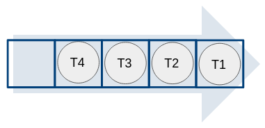
The O(1) scheduler creates a new queue (linked list) for each of these 140 different priority values. For the real-time tasks (queues 0-99), processes within each priority list are scheduled either FCFS or RR, which can be toggled by the user (look for SCHED_FCFS and SCHED_RR). The user-space tasks (100-139) are typically scheduled RR per priority (SCHED_NORMAL) but they can also be scheduled based on remaining runtime to improve batch processing (SCHED_BATCH). Each priority list is emptied in full before the next priority list is considered. At every context switch (at every time slice), the highest priority list with a runnable task is selected.
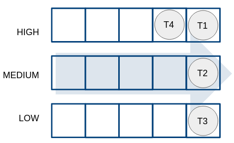
If we were to use this setup directly, the lower-priority tasks would very often by interrupted by higher-priority ones and we again get the problem of starvation. To prevent the need for manual priority adjustment with ageing, the O(1) scheduler instead uses a clever trick, by introducing a second, parallel datastructure. As such, there are two groups of 140 queues. The first is called the “active” queue, the second the “expired” queue. When a task has consumed its time slice completely (either in 1 run, or by yielding multiple times), it is moved to the corresponding “expired” queue. This allows all processes in the active queue to get some time. When the active processes are all done, the expired and active lists are swapped and the scheduler can again start with the highest priority processes.
This setup is efficient, because we no longer need to loop through all tasks to find the next one: we just need the first task in the highest priority list! As long as processes are added to the correct priority queue, this can be done in constant time. Some psuedocode to illustrate these aspects can be found below:
// pseudocode!!!
// in reality, the data structures and functions look different!

struct PriorityTask {
    struct Task *task; // for example the PCB
    struct PriorityTask *next;
}

struct PriorityList {
    struct PriorityTask *first;
    struct PriorityTask *last;
}

struct RunQueue {
    struct PriorityList *tasks[139]; // 140 linked lists, 1 for each priority
}

void appendToList(struct PriorityList *list, struct Task *newTask) {
    // TODO: make sure list->last exists etc.
    list->last->next = newTask;
    list->last = newTask;
}

struct RunQueue *active;
struct RunQueue *expired;

// new task is started with priority x
appendToList( active->tasks[x], newTask );

// scheduler wants to start a new task
// loops over "active->tasks" from 0 to 139, looking for the first non-empty list, with index y
// Note: in reality, a bitmap is used to prevent the need to loop (see below), keeping things O(1)
struct PriorityTask *runTask = popFirstFromList( active->tasks[y] );
execute( runTask->task, runTask->task.timeslice )

// task is done running and has consumed its timeslice completely
appendToList( expired->tasks[x], runTask );

// OR: task is done running and hasn't consumed its timeslice yet (waiting state)
runTask->task.timeslice = leftoverTimeslice;
appendToList( active->tasks[x], runTask );

// if all lists in "active" are empty (no "y" found): swap both runqueues and start over
struct RunQueue *temp = active;
active = expired;
expired = temp;
How would you implement appendToList and popFirstFromList in practice? What other properties should struct Task have besides “timeslice”?
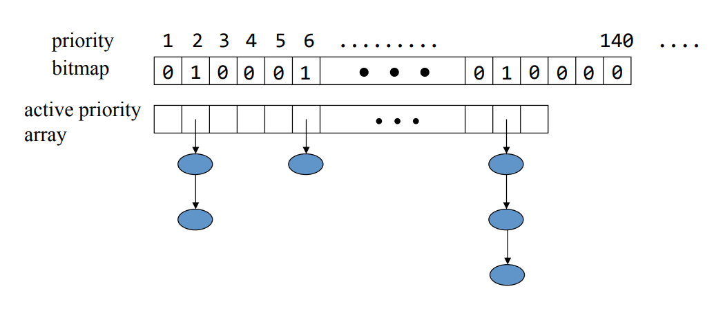
As explained in the pseudocode, we also need a clever way of knowning which priority queue still has pending tasks without looping over all of them. This can be cleverly done by using a so-called bitmap, where each individual bit of an integer is used as a boolean to indicate if there are tasks for the priority corresponding to that bit. To represent 140 bits, we need about 5 32-bit integers (total of 160 bits). Checking which bits are set can be done very efficiently. See the image below for a schematic representation:
As such, we can see the O(1) scheduler is an excellent example of a complex multi-level feedback queue! It utilizes several queues for the different priorities, using different schedulers per-queue depending on the real-timeness of the task. On top, it has two higher-level queues (active and expired) for which it uses an FCFS scheduler. Conceptually a different time slice could also be employed (e.g., higher priorities get a longer time slice), though this was typically not employed.
This scheduler is however not perfect. In practice, it turns out that I/O-bound or interactive processes could get delayed considerably by longer-running processes, due to the active vs expired setup. This caused the need for a complex set of heuristics (basically: educated guesses) that the OS would use to estimate which processes were I/O-bound or interactive. These processes would then receive an internal priority boost (again a form of ageing), while non-interactive processes would get penalized. In practice however, like with the O(n) scheduler, this process was somewhat unstable and error-prone.
The Completely Fair Scheduler
The current default scheduler was intended to take a bit of a step back from the relatively complex O(1) scheduler and to make things a bit simpler; as we’ll see however, that’s simpler for Linux kernel developers, not necessarily for us. The CFS is a relatively complex scheduler, and as such a thorough study on this algorithm falls out of the scope of this course. We will touch upon the main concepts however.
The main insight in the CFS is that the size of the time slices can be highly dynamic. Previously, we’ve seen that interactive processes for example can get 8ms, while CPU-bound processes could get 16ms. That’s already nice, but it doesn’t take into account the current load of the system: if there are many different processes waiting, each will still get 8 to 16ms, causing later ones to be significantly delayed.
The CFS solves this problem by calculting the per-task time slice length for a given time period based on the number of ready tasks. Say that N tasks are ready and we want to schedule each of them over the next 100ms (an “epoch”). Then each task is assigned a time slice of 100ms * 1/N (if we ignore the context switching overhead for a bit). In theory, this gives each task an equal share of the processor, hence the name. As such, if there are fewer tasks active in the system, N will be lower, and the time slices will get larger, and vice versa. Of course, the CFS puts a lower bound on the time slice length (typically 4ms) as otherwise the context switching overhead could become too large.
To determine which task executes first within the next epoch, the CFS keeps track of how much time each task has actually spent on the CPU so far. As such, for I/O-bound processes that yield frequently, this value will be lower than for CPU-bound tasks that always use their full time slice. The scheduler always selects the process that has so far spent the least amount of time on the CPU. This automatically makes sure that interactive processes are scheduled frequently enough, but also that CPU-bound processes age correctly.
This timekeeping is done in a quite complex datastructure called a (binary) (self-balancing) red-black tree. The details are not important here, but this mainly means that the next task (that has spent the last amount of time on the CPU) is always the most bottom left node in the tree. As such, it can easily be retrieved with low overhead. Similarly, adding new tasks (or moving tasks around) in the tree can be done in O(log N).
The complexity increases even more when we look at how this setup incorporates priorities. As there are no longer explicit per-priority lists like in the O(1) scheduler, the CFS simulates this by shrinking/expanding the time slices of low/high priority processes. This is similar to what we’ve discussed above, that time slice durations can be used to emulate priorities. As such, if a high priority process executes for 10ms on the CPU, the timekeeper might only record that it spent 5ms of “virtual time”. This gives the task a “priority boost” when the scheduler next goes looking for a new task. The opposite is done for low priority tasks (e.g., 10ms of runtime can become 20ms of “virtual time”). We can see this is no longer a “completely fair” scheduler in practice, but it’s quite elegant in how it combines interactivity, priorities and time slice lengths in practice.
For more information on CFS you can read the kernel documentation here. For the daredevils … you can even read (or modify, at your own risk) the kernel C code here.
Other schedulers
As might be expected, these are not the only schedulers that exist, even within Linux. There a many schedulers available and, certainly, there will be many more to come. Just a small grasp of existing schedulers:
- Brain F*ck Scheduler (Linux)
- Noop Scheduler (Linux)
- Task Scheduler 1.0 (Windows)
- Task Scheduler 2.0 (Windows)
- JobScheduler (iOS)
Look up at least 1 other scheduler (for example one used in Windows) and grasp its main concepts and compare it to how Linux works.